Introduction

In previous papers (1) a thought experiment started with generalizing the physical forces (starting with gravity) and the evolutionary forces (starting with plant growth), just because they show a second order polynomial in the direction of time. Such a generalization is justified if we try immediately to find falsifications (2). Successive papers ( see 4 and 5) tried to do this but did not succeed right away. Other people, preferably physicists with a suitable track record, are challenged to help. The author tries in this paper (almost deliberately to end the crazy experiment), to force falsification in a new way by showing that in the early used simulations with 2-dimensional plants, as simple as possible, it is not possible to break symmetry and to create a simple, winning superposition, two phenomena so important in physics. Actually they are details in falsifying the whole idea by the Quantum Theory, see 6.

If, by surprise, this falsification would not succeed, we would still have another falsification which should certainly succeed: Some kind of entanglement of the in evolution successfully emerging super positioned 2-dimensional plants seemed really impossible.

Methods

We used the methods described in (7), (8), and (9), where we showed that simulated two-dimensional plants, as simple as possible, win when they grow according a polynomial of the second order. It was the trigger for a provocative thought experiment mentioned in the introduction.

We introduced in (10) for a falsification a new type of plants, i.e. with bended leaves instead of horizontal leaves see figure. Notice the plants are symmetrical if we consider two directions for the leaf. The axis of symmetry is the stem of the plant.

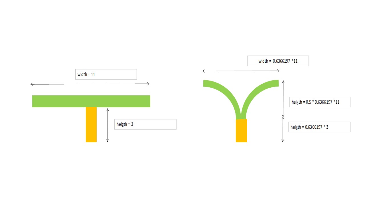
Figure 1: Symmetric, simulated, two-dimensional plants, as simple as possible, with horizontal and bended leaves, respectively

We here added other type of plants: plants who had one leaf in one direction, see figure 2. The symmetry is broken. We wanted just see if they would survive.

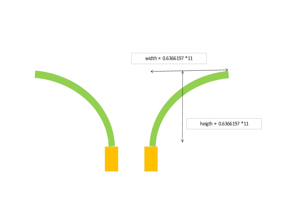
Figure 2. : Asymmetric, simulated, two dimensional plants, as simple as possible

The evaluation of the competition was in most cases again the same as with symmetric plants. If a plant was lower than the adjacent plant, it was supposed to be overshadowed in the next time steps, and to lose. It was eliminated, even if the overshadowing was just starting, see figure 3.

Figure 3. Wins and losses in the evaluation of competition between simulated two-dimensional plants, as simple as possible, with bended leaves, when one the two is loosing

We formulated one draw in the mentioned, previous simulated experiments: When two plants were touching each other, while having the same height, they were supposed to reproduce and die in the same timestep (the most simple solution). See the left part of figure 4.

We had to formulate one extra draw, see the right side of figure 4: If two plants have both one leaf, pointing in the same direction, one plant can only touch the other with a leaf. If this plant is smaller than the touched plant it cannot overshadow the other plant. So, it cannot win. The other cannot win either because it has not a leaf on the side of the former plant to overshadow it. Therefore, we had to decide for a draw: Again both die and reproduce.

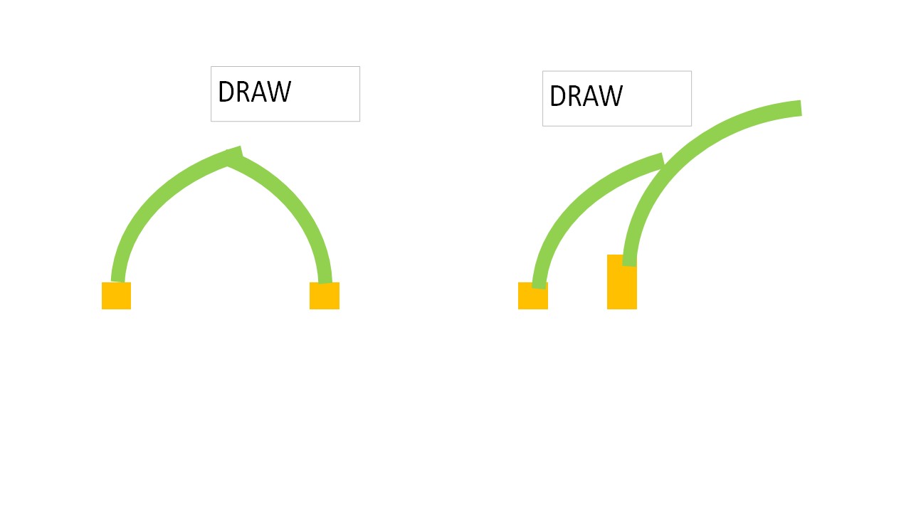
Figure 4: Draws in the evaluation of competition between simulated two-dimensional plants, as simple as possible, with bended leaves. On the left side the usual draw (2 plants with the same hight), on the right side two plants with one leaf in the same direction, where the touching plant cannot win because it is smaller.

Next, there was the realization that you could differentiate in the reproduction in the asymmetric plants, i.e. the plants with one leaf, creating a superposition:

Plants producing only descendants with a leaf in the same direction of the mother plant. We called these plants “with not super-positioned descendants”
Plants producing descendants with a leaf randomly in one direction. So, in the population we created some kind of superposition. We call these plants “with super-positioned descendants”.

Suddenly ,there was the second realization: The “super-positioned descendants” gave the possibility of some kind of entanglement:

Plants where the superposition is, as stated, randomized: The direction of the leaf of a descendant is randomly chosen.
Plants where the superposition is entangled: if the direction of the leaf of a descendant is in one direction, then the direction of the leaf of the next descendant is in the other direction.

Summarizing, we had to test against each other (In parentheses are the abbreviations the parameters and their values of used in the rest of the paper):

Symmetric plants (SYM = y(es))
Asymmetric plants (SYM = n(o))
1. with not super-positioned descendants (SUPERP = n(o))
2. with super-positioned descendants (SUPERP = y(es))
  1. with randomized direction of leaves (DIRL = r(andomized))
  2. with entangled direction of leaves. (DIRL = e(ntangled))

Important parameters found in previous experiments were taken into account (In parentheses are the abbreviations used in the rest of the paper):

Order of the polynomial describing growth (ORDGR = number)
maximal age (MAXAGE = number)
The minimum ratio between an amount of a factor in a plant and an amount of the same factor in a second plant to make the first plant win (MINRAT = number).
Introduction of other factors then height vs no introduction (INTRFACT = n(o) ore y(es)).

We let values of one parameter compete with each other, while keeping the others constant.

We started always with one plant having one value and a second having another value for the competing value with two exceptions:

The competition between polynomials of different order started with one having the third order, followed at some point by introduction of the second order
The factors other than height were also introduced at some point

Notice, in an earlier experiment (8, see 5.3)), where we showed that second order polynomials reappeared as winning form third order polynomials in plants with bended leaves when other competition factors were introduced, we started with secondary part consisting for 100% of factor 1, so no height. In this experiment the secondary part consists at the start for 100% of height. The reason was that height was important for evaluating the superposition and related entanglement.

The simulated 2-dimensional planting area consisted of 250 elements.

A preliminary experiment was necessary to establish that the most favourable maximal age was for the second order polynomial plants 7 and for the third order polynomial plants 9.

Next, one experiment was conducted:

Asymmetric plants with “non super-positioned descendants” against asymmetric plants with “super-positioned descendants”.

Then it turned out that we needed 12 experiments (in at least 4 replications) to describe what can happen with asymmetric against symmetric plants and entangled against non-entangled plants in a 2-dimensional simulated area, as simple as possible. Actually there were a lot more experiments, but the 12 are necessary to present clear results.

Results

Experiment 1 showed that asymmetric plants with not super-positioned descendants lose very fast from asymmetric plants with super-positioned descendants. It was the reason to use in other experiments only asymmetric plants with super-positioned descendants.

The relevant 12 experiments presented in table 1 gave the relevant results.

Table 1: Results of experiments primarily testing asymmetric, super-positioned against symmetric plants and entangled against non-entangled plants and secondly how these test are influenced by other factors as order, growth, optimal maximum age and minimal ratio to win

Nr.	ORD GR	MAX AGE	INTR FACT	MIN RAT	SIM	SUP POS	DIR LF	RESULT
2	2-3*	9	y	3	Y	Y	–	Polynomial order 2 wins from order 3 in 3 out of 4 cases
3	2-3**	7	y	3	Y	y	–	Polynomial order 2 wins from order 3 in 3 out of 4 cases
4	2	7	y	3	y-n	y	R	Asymmetric loses from symmetric in 4 out of 4 cases
5	2	7	n	3	y-n	y	R	Asymmetric wins from symmetric in 4 out of 4 cases
6	2	7	n	3	N	y	r-e	Entangled loses from not entangled in 3 out of 4 cases
7	2	7	n	1.1	N	y	r-e	Entangled wins 11 out of 15 cases
8	2	7	n	1.1	y-n	y	E	Asymmetric wins from symmetric in 4 out of 4 cases
9	2	7	y	1.1	y-n	y	E	Asymmetric wins from symmetric in 4 out of 4 cases
10	2-3	7	y	1.1	N	y	E	Polynomial order 2 loses from order 3 in 4 out of 4 cases
11	3	7	n	1.1	N	y	r-e	Entangled wins from not entangled in 5 of 10 cases
12	3	9	n	1.1	N	y	r-e	Entangled wins from not entangled in 4 out of 4 cases
13	3	9	n	1.1	y-n	y	E	Asymmetric wins from symmetric in 4 out of 4 cases

* We had to increase the rate of introduction of second order plants in an area full of third order polynomial plants from 5% to 10% to get the second order polynomial at least a 50% share. The introduction of new factors was then only started and the rate of introduction was also raised to 10%. It was only then possible for the second order polynomial plants to win.

** idem

A side discussion in this paper is the fact, see the asterisks and accompanying remarks in experiments 2 and 3, that it is not easy to let win the second order polynomial plants form the third order polynomial. One explanation is that we started with a secondary part consisting for 100% consisting of height. This benefits third order plants which are already in favour with height by the bending of the leaves giving them production ability as well as competitive ability (). Still, there is reason to assess once again the idea that plants growing according a second order polynomial win from those growing according a third order polynomial in an highly competitive (a lot of factors) area.

But the main focus was, as stated in the introduction, the question if breaking symmetry, superposition and entanglement was in some kind possible in 2-dimensional simulated plants, as simple as possible.

As a big surprise, the answer is yes. Table 1 shows when:

In experiments 2 and 3, second order polynomial plants replace third order polynomial by rapidly introducing new competing factors (INTR FACT = y), while height is only winning when it is 3 times higher than the competing neighbour (MIN RAT=3). In that situation symmetric and therefore not-entangled plants have the advantage, see experiment 4.
In experiment 5 with no introduction of new factors (INTR FACT = n), suddenly asymmetric plants win.
In that case, see experiment 6, entanglement loses from non-entanglement
This changes, see experiment 7, when height was made more important, i.e. when the plant is already winning being 1.1 times higher (MIN RAT=1.1). than the competing neighbour. Entanglement is suddenly winning in most cases.
Experiments 8 and 9 are just checks if asymmetric is still winning. It is.
In that situation third order polynomials are winning, see experiment 10 and this increases the winning of entanglement, see experiment 11, in particular when we change to the winning maximal age (MAX AGE = 9) for third order polynomials, i.e. 9, see experiment 12.
Experiment 13 is again a check if asymmetric is still winning. It is.

Discussion

The evaluation is as follows:

Experiment 1 (super positioned is in favour in asymmetric plants) : The possibility of attacking in both directions will give an advantage over attacking in only one direction. More draws in both directions versus less draws in one direction, see the explanation for experiment 5, will add to this advantage
For the possible explanation of experiments 2, 3, 4 (symmetry is in favour) you need the possible explanation for experiment 5 (asymmetry is in favour): There the winning of asymmetric plants with superposition from symmetric plants could be due to the fact that the asymmetric plants produce more draws, see right part of the figure 4. Maybe they have less inner competition in a population and can they concentrate on the external competition. Further research is necessary. Notice, this is only applicable to the competition by height with the concept of overshadowing. This is not the case for the other factors. It gives the possible explanation for the winning of symmetric plants in experiments 2,3, 4, when factors are introduced at an high rate and height is given a less important role, i.e. only winning at a ratio of 3 (MIN RAT = 3).
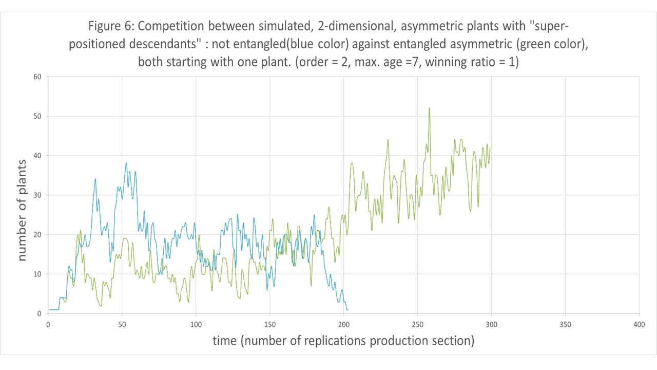
Why entanglement loses in experiment 6 and wins in experiment 7 is not clear. Height was made more important in experiment 7, getting more competitive ability with a ratio of 1,1 (MIN RAT =1,1). It resulted in a less dense population of appr. 40 plants (see figure 5) instead of appr.140 plants in experiment 6 (see figure 6). Maybe in a less dense population the plants have to assure that there is an exact balance between right and left oriented asymmetric plants, that entanglement is necessary. But if this is not important in dense populations, see experiment 6 (the difference in amount of right and left oriented plants will be much less), why do randomly left or right oriented asymmetric plants win? Why does a mix not survive? And why is in that case the change of survival not 50% for both types of plants? Is a slight disturbance in the equilibrium by non-entanglement favourable in dense populations to escape and make plants older and let them kill a lot of entang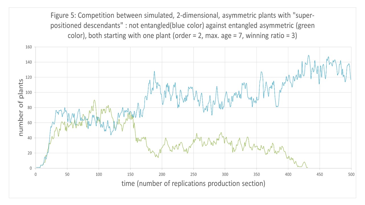led plants in experiment 6? Research is necessary.

Experiments 8,9 and 13 are, as said, just tests if asymmetric plants are still winning from symmetric.
Experiments 10 showed once again that , when height wins at a lower ratio (MIN RAT = 1,1), third order polynomial plants win from second order polynomial plants.
In that situation (MIN RAT = 1,1), third order polynomial plants with entanglement win from those without in 50% of the cases, see experiment 11, and in 100% of the cases when the maximal age is optimal for third order polynomial plants, i.e. 9 . The speculative explanation is the same as for the second order polynomial plants, see experiment 7, the density of the plants was appr. 60 in experiment 11 and 40 in experiment 12.

Conclusions

In the end, the generalization of the physical and evolutionary forces is not falsified in these experiments with 2-dimensional, simulated plants, as simple as possible: Some kind of breaking symmetry, superposition and even entanglement is possible in evolution; they give in the right combination even an evolutionary advantage over symmetry.

There seems a tendency. In case of an high mutation rate symmetric, second order polynomial plants are the survivors, but if the rate lowers asymmetric, entangled, in vigorous growth exploding third order polynomial planta are the survivors.

So, the “crazy” thought experiment is to be continued.