Previous papers (link1, link2) showed plants not to grow exponentially, as many scientists expect at least until 1990 (link3), but according a polynomial of the second order.

To explain why a plant would not grow exponentially, we have to leave the basic idea of exponential growth i.e. that the ratio of the growth machinery in plant mass stays the same (Thornley, 1990). It implicates that we have to divide the total plant mass in growth machinery and non-growth machinery. In this article the terms productive mass and unproductive mass are preferred. So, we have the equation:

y = y_P + y_NP                                                                             (1)

Where

y          = total plant mass                                                     (mass)

y_P         = productive mass                                                    (mass)

y_NP        = unproductive mass                                              (mass)

The productive mass is defined, using the idea of the growth machinery as follows:

Productive system = the part of the plant that uses its mass (energy) only to fix more mass (energy) for the plant.

It is the photosynthetic system in a plant.

The unproductive mass has to have also a function in the Darwinist vision, as the survival of the fittest blocks every waste of energy. If it does not contribute to energy fixation, it must contribute to competition ability ore competition avoidance. It leads to the following definition:

The unproductive system = the part of the plant that uses its mass (energy) for competition ore competition avoidance.

E.g. a plant has avoided the competition of only in water living organisms by establishing itself on land and in the air. But it invests necessarily a lot of its energy in systems for transport of water and nutrients out of the soil to its light intercepting leaves in the air. Other energy goes to direct competition, e.g. to the production of for other organisms poisonous substances.

The implication of the division of the plant in these two parts is a change in the master equation of exponential growth. The gross growth rate is no longer linearly related to the total plant mass but to the productive plant mass. So

P = Cy_p                                                                                         (2)

Where

y_p         = see eq. 1

P          = gross growth rate of a plant                                    (mass time^-1)

C          = relative growth rate of the productive mass       (time^-1)

Of course, the objective of this paper is the description of the net growth rate. A universally accepted equation relating the gross production to the net production is the following one, where the loss is attributed to respiration:

dy/dt = P – R                                                                                  (3)

Where

y,t, P    = see eq. 1, 2

R          = respiration                                                                   (mass time^-1)

Next, the respiration is described by the following relation (Thornley, 1990):

R = r dy/dt + m y                                                                         (4)

Where

y,t,R     = see eq. 1.2 and 3

r           = growth respiration parameter                                ( – )

m         = maintenance respiration parameter                      (time^-1)

The description of the net growth rate becomes very interesting, if, first, P and R are replaced in equation 3 using equations 2 and 4, which describe them in productive plant mass and total plant, mass, respectively.

dy/dt = Cy_p  – (r dy/dt + m y)                                                    (5.A)

or

(1 + r) dy/dt = Cy_p  – m y                                                            (5.B)

or

dy/dt = (Cy_p  – m y)/(1+r)                                                            (5.C)

Where   y, y_p,t, C, r, m    = see eq. 1, 2, 3,4

R          = respiration                                                                          (mass time^-1)

Secondly, y is replaced in de right side of the equation by the sum of the productive and unproductive mass (see equation 1). The goal is clear: The growth rate should be expressed as a change in balance between the productive and the unproductive mass, as this is the reason for the non exponential growth.

dy/dt = (Cy_p  – m (y_P + y_NP))/(1+r)                                             (6.A)

or

dy/dt = ((C – m)y_p  – my_NP)/(1 + r)                                             (6.B)

This is with a = (C – m)/(1 + r) and b = m/(1 + r)

dy/dt = ay_p  – by_NP                                                                        (7)

This equation opens an interesting possibility, when we use the observation that the relation between the plant mass and time is a polynomial of the second order. It implicates that

dy/d²t =  constant = f                                                                   (8)

Thus, combining 7 and 8:

d(ay_p  – by_NP ) = constant = f                                                      (9)

Suddenly we have a very exact quantification of how exponential growth changes to second order polynomial growth by a change in the balance of productive and unproductive growth. The difference between the growths of both should be constant (considering the two parameters a and b).

So, there is a simple model for growth according a polynomial of the second order.

Notice that y_p  and y_NP will grow also with the square root of time.

The derivative of equation 1 is:

dy = dy_P + dy_NP                                                                            (10.A)

or

dy_NP  = dy – dy_P                                                                            (10.B)

replacing  dy_NP in equation 9 gives:

(a+b)dy_P  = bdy + f                                                                        (11)

Next, replacing dy_P in equation 10.B gives:

(a+b)dy_NP  = ady – f                                                                      (12)

So, knowing that a,b en f are constant, author’s knowledge of mathematics say that equations 11 and 12 indicate that dy_P  and dy_NP have the same behaviour as dy.

But the author possesses a more elaborative discussion of this model which shows the stability of the solution. It shows even that for a function f(t) of the N order the mass y(t) behaves like a polynomial of the N + 2 order.

As this discussion is the product of another author, who did not give permission to publish and does not support the reasoning in this series of papers, this paper is only challenging other interested persons to proof the (un)stability of the solution.

We changed this model of differential equations to one of difference equations to make it possible to use it in computer simulations. We did not notice any important changes in the main characteristics. See Appendix.

References

Thornley, J.H.M. and I.B. Johnson, 1990. Plant and Crop  Modelling: A mathematical Approach to Plant and Crop Physiology. Clarendon, Oxford.

APPENDIX: The same model with difference equations

 

In the paper above we described a model which could explain growth according polynomials (1 ^st , 2^nd , 3^rd order, etc). We used there differential equations. For computer simulations we use difference equations, we did not encounter any important changes in the characteristics.

So, equation 1 about the partition in productive and unproductive (competitive) mass becomes:

y_(t) =   y_P(t) +  y_NP(t)                                                                    (1 difference)

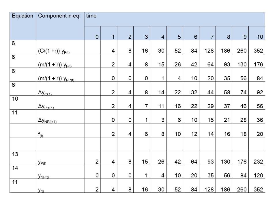
See last 3 rows in tables 1,2 and 3, where we simulated 1 ^st , 2^nd , 3^rd order growth for  plants, as simple as possible,. On t=0 the values are initialized. We chose:

y₍₀₎ = 2

y_P(0) = 2

y_NP(0) = 0

Equation 6B, expressing the net growth as the gross production corrected for the growth respiration and diminished with the maintenance respiration of both the productive and unproductive mass becomes:

Δy_(t+1) =  (C/(1 +r)) y_P(t) – (m/(1 + r)) y_P(t) – (m/(1 + r)) y_NP(t)   (6B difference)

See for the components on the right side of the equation the first 3 rows in tables 1,2 and 3. The left side of the equation, the net growth, to be calculated from these components is in row 4. We only need to choose values for the parameters. We choose convenient numbers:

C = 4

m = 2

r  = 1

Of course, we can get y_P(t) and y_NP(t+1) from rows 9 and 10 from the previous time step (column)

The way this growth rate can be partitioned in productive and unproductive mass is described by equations 10 and 11. They become as difference equations:

Δy_P(t+1) =   (m/C)Δy_{(t + 1)} +  ((1 + r)/C) f_(t)                    (10 difference)

Δy_NP(t+1) =   (m/C)Δy_{(t + 1)} –  ((1 + r)/C) f_(t)                   (11 difference)

See rows 5 and 6 of the tables. C, m and r were already chosen. We decided f_(t) to be for

First order:       f_(t) = 0

Second order:  f_(t) = 2

Third order:       f_(t) = 2t

De new total mass, productive and unproductive (competitive) mass are by definition:

y_(t+1) =y_(t)+Δy_(t+1)

y_P(t+1) = y_P(t) + Δy_{P(t + 1)}

y_NP(t+1) = y_NP(t) + Δy_{NP(t + 1)}

So we can calculate in each time step (maximum = 10) the new mass and the partition over these two essential components.

Table 1: Simulation of simple plants growing according a polynomial of the 1^st order, caused by no difference (f_(t)  = 0) in growth rate of productive and unproductive (competitive) mass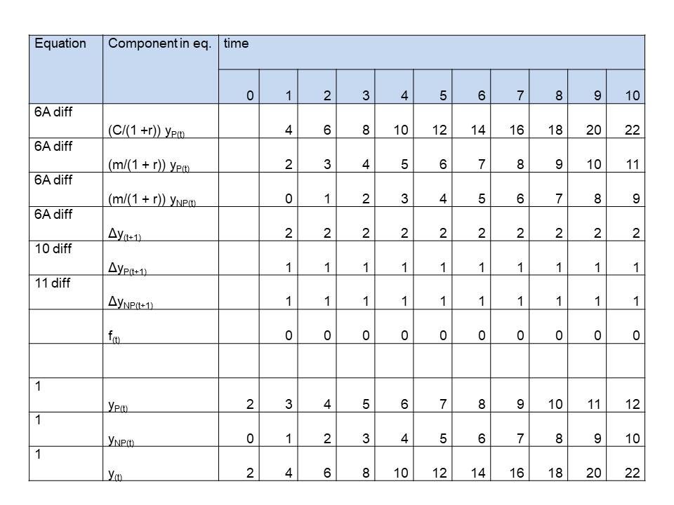

Table 2: Simulation of simple plants growing according a polynomial of the 2^nd order, caused by a constant (f_(t)  = constant = 2) difference in growth rate of productive and unproductive (competitive) mass

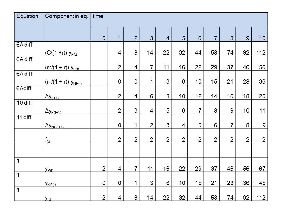
Table 3: Simulation of simple plants growing according a polynomial of the 3^rd order, caused by a linearly with time increasing difference in growth rate of productive and unproductive (competitive) mass (f_(t)  = 2t)

Where

y_(t)        = total mass at time = t

y_P(t)         = productive mass at time = t

y_NP(t)     = competitive mass at time =  t

Δ          = growth in timestep  = 1

C          = relative growth rate not corrected for growth rate = 4

r           = correction for growth respiration = 1

m         = maintenance respiration = 2