Introduction
Experiments (link1, link2) indicate that plants do not grow exponentially but according a second-order polynomial. In an earlier paper (link3) is described how a n-order polynomial is derived from an exponential model. The essence of the reasoning is a shift from the growth machinery to more competitive ability. The question remained why a plant, growing according a second-order will win in a struggle for survival from those not growing according these characteristic.
To find an answer a computer simulation was made where plants growing according a second-order were competing with slower growing (accordinga first-order polynomial) plants. In a second paper (link4) we will evaluate the competition with faster growing (according a third-order polynomial) plants.
Methods
The computer simulation was written in Visual Basic and the results of each time step was recorded in Excel sheets. It was a simple as possible to avoid too much complicating factors. The assumptions are (see also Figure A):

Figure A: Simulated two-dimensional plant
- The growth space is two-dimensional, a torus of 1000 cells.
- The plants are therefore also two-dimensional. It has one leaf represented by one horizontally row of cells (see figure A green cells). It is as big as the simulated productive mass is at that moment. It has one stem represented by one vertical row of cells (see figure A, yellow cells). It is as big as the simulated unproductive mass is at that moment. The end of the stem is fixed to the middle of the leaf. So the leaf is growing for one half to one side and for the other half to the other side each time step.
- The two-dimensional plants are randomly placed in the space.
- The energy is supposed to come from above. So it will intercepted by the leaf. Other substances are supposed not to be necessary for the simulated plant. Notice that it is easy to make a mirror image of the plant and to suppose that water and nutrients are coming from under and that there is an absorbing surface like the leaf and a transport system like the stem. Then the simulated plant is more real plant. It won’t change the results of the simulation.
- The mean transport length from the productive to the productive mass increases when the plant grows. It implies extra transport tissue. It is assumed to be part of the unproductive mass. It means that each unit of the unproductive mass produces less height. It is assumed to be negligible up to the maximum age used in this experiment.. It is necessary to avoid a disadvantage for faster growing plants from the beginning.
- The influx of energy is evenly distributed over the torus.
- The competition is evaluated when the plants touch each other.
- The mechanism for evaluation is as simple as possible. The plant with the greatest unproductive mass, i.e. the greatest stem, i.e. the highest plant, wins. It is supposed to overshadow the other plant. The evaluation is after each time step. All possible touching between plants is evaluated. So, not only plants who are standing side by side are evaluated, but for each plants all plants in reach of it’s leaf surface (productive mass) are evaluated. In Figure B this evaluation is illustrated. The at the moment of evaluation losing plants are indicated with a red cross. The red arrows show the plants who are causing the damage.
- The plants grow according either a first-order or a second-order polynomial. The exact models are given in the appendix from an earlier paper (link3). We introduced only one extra time step at the beginning. For all models we start from one cell and we let them double in the first step to two. It is necessary to start from one unit.
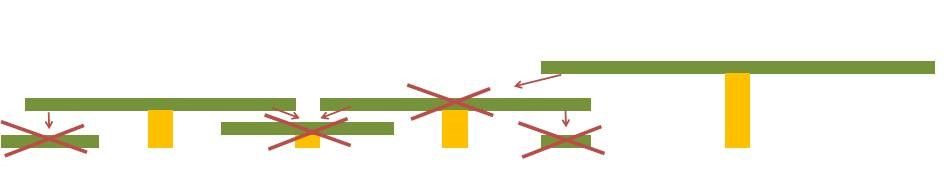
Figure B: Competition evaluation of simulated plants.
There emerged inevitably other complicating factors:
- The first reasonable assumption is that a plant dies after a certain period. We discovered to our surprise that there is an optimal time to die, a maximum age, depending on the growth pattern. We prepared a separate paper to discuss this interesting phenomenon, see (link5). We chose in this competition experiment the optimal maximum age of the first order growth, to put the second order growth not in a favourable position. The plant can die earlier by loosing the competition.
- The second reasonable assumption is that the plant tries to reproduce for it dies. In this experiment it is again as simple as possible. The amount of offspring is as big as the production of the mass would be in the next time step after death.
- A decision was needed on what should happen with a draw, i.e. when to plants would have the same height (= the same unproductive mass) when they touch each other. Again, the requirement is that the simulation is as simple possible: The plants die and reproduce both. Complicated evaluation mechanisms are necessary in other cases.
- Finally, a decision was unavoidable on what should happen when offspring (seed) is placed in cells already occupied with seed. It is reasonable is to evaluate the dormancy. The incoming seed will replace the seed already there if the dormancy is shorter.
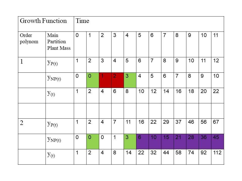
Notice that a plant investing more than a second plant in its productive mass, i.e. more in the growth machinery, and less in its unproductive mass, i.e. its competitive ability, will have after a while also a bigger unproductive mass in absolute terms. It overtakes the second plant in competitive ability after an initial gap by its bigger production capacity. (see table 1). However, the question is whether the plant can achieve the higher ages, when competition is intensive.
Tabel 1 : Productive mass (yP(t)), unproductive, competitive mass (yNP(t)) and total mass (y(t)) as function of time of plants growing according a polynomial of the first order and the second order. The colour dark red and dark purple indicates the winning order polynomial at that moment: The competitive mass is bigger, i.e. the stem is higher. Dark red is for the plants investing initially more in competitive ability and purple for the plants investing initially more in production. The color green indicates a draw.
The program had switches to introduce mutants:
- Offspring could change for a certain percentage from growing according a x-order polynomial to an y-order polynomial.
Two simulations were conducted:
- The first experiment started with only one plant. The growth characteristic was a second-order polynomial with random distribution of the seeds over the space of the torus and over the dormancy period from 0 to maximum age (10). It was allowed to grow and multiply to a high density. It means maximal competition. After a certain period we introduced with a mutant switch plants growing according a first-order polynomial. The switch was set off, when the amount of the mutants reached a percentage far above 50. So, the second-order polynomial plants, the expected winners, have at that moment a disadvantage in numbers.
- The second simulation was the same as the first one, only there was not a random distribution of the seeds over the whole space over the dormancy period. They were concentrated around the mother plant and around a dormancy time of 0 according a distribution function.
Results and Discussion
(14-8-2020: Notice, the results were corrected as a mistake in the programming caused that only the right side of the plant was competing. It was corrected without making a separate publication, because the main conclusions stayed the same . Moreover, it emphasizes the robustness of the conclusions. Only some numbers changed.)
The results of the first experiment are disappointing for the second order plants when the offspring is randomly distributed in space and time. See figure 1: After getting the possibility to establish itself over the whole area in period 1, they loose from first order plants when these are introduced at a rate of 5% in period 2, even when the mutations stopped in period 3. Notice that we used the optimal maximum age for first order plant , i.e. 2, see paper (link5).
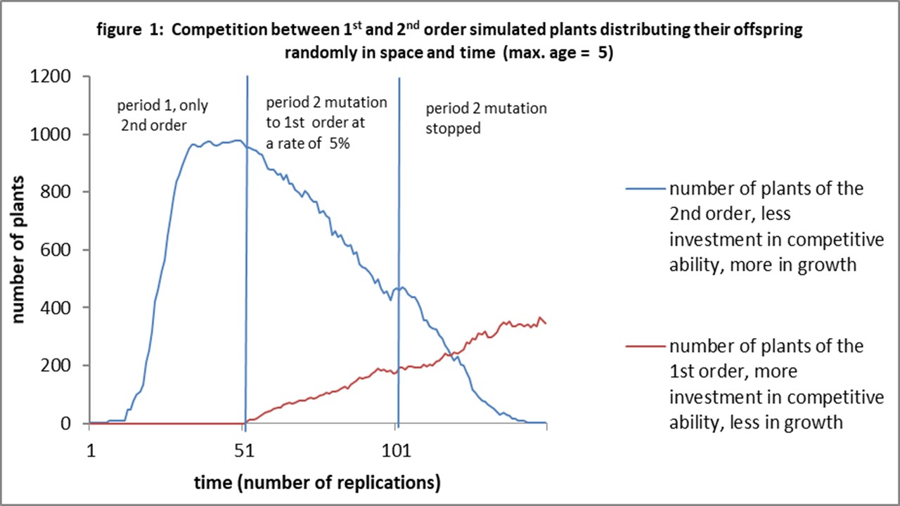
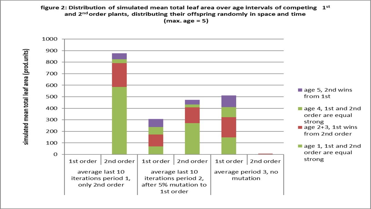
Figure 2, trying to reveal the mechanism by assessing the leaf area per age, shows more first order plants winning from second order plants (age 2 and 3) than vice versa (age 5) at the end of period 2.
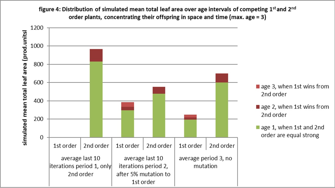
This seems obvious, but figure 3 and figure 4 show a more subtle mechanism. When the plants concentrate their offspring in time (see also paper link6), the second order plants win suddenly from the first order plants, but not by having more plants winning at favorable ages. There is a shift a in optimal maximum age for the first order plants when concentrating, i.e. from 5 to 3 (see paper link5). That implies that there is no age were the second order plants win. Now we are wondering: Why they still win?
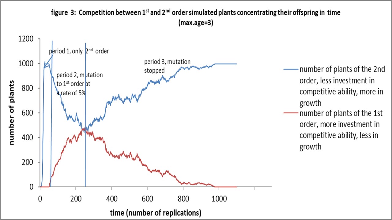
The only explanation of the author is: Look at the reproduction rate. It is higher for the second order plants at ages 2 and 3. If they are not attacked fast enough their population will grow faster. Notice, concentration implies a bigger internal competition for plants of the same order. They will kill each other more. The competition with populations of the other order is more at the border. The population with a higher reproduction can recover faster and not only avoid empty spaces in their own population, but can also occupy faster an empty space provided by internal competition of the less faster reproducing population.
So, the advantage in competitive ability is not enough to compensate at least for the disadvantage of the much lower production and reproduction.
The next question is which situation will occur more: Plants who concentrate their offspring in time and space giving an advantage for 2nd order plants or plants who do not, giving an advantage to 1st order plants. Another paper (link6) shows that plants concentrating their offspring win from who don’t.
So, without being a formal proof, this simulation supports the idea that plants will grow rather according a second order than according a first order, i.e. slower growth.
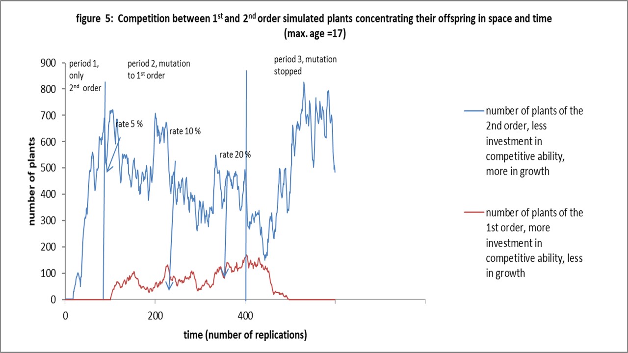
Notice, that at the optimal maximum age of second order plants, i.e. 17, the first order plants are without a change, see figure 5. We have to raise the mutation rate to 20% to get more first order than second order plants. See also the low coverage of the area by the first order plants. It shows again that the competition between the first order plants themselves (intra competition) and their low reproduction rate cause empty space.